TCGA-BRCA guided tutorial

1.Setup the Linkage Object

For this tutorial, we will be analyzing the dataset of Breast Cancer (BRCA) freely available from TCGA. The dataset contains chromatin accessibility and gene expression data from 72 patients with BRCA, which can be load from LinkageData. You can also found the raw data from here.

We start by loading in the data. The BreastCancerATAC() and BreastCancerRNA() function can load and return the available chromatin accessibility and gene expression matrices from Linkage. The chromatin accessibility matrix is a normalized bulk ATAC-seq count matrix, which a prior count of 5 is added to the raw counts, then put into a "counts per million", then log2 transformed, then quantile normalized. The gene expression matrix is a normalized bulk RNA-seq count matrix, which is log2(fpkm+1) transformed.

We next use the chromatin accessibility and gene expression matrix to create a Linkage object. The object serves as a container that contains both data (like the count matrix) and analysis (like regulatory peaks, or active TFBS).

library(Linkage)
# library(LinkageData)
# ATAC_count <- BreastCancerATAC()
# RNA_count <- BreastCancerRNA()
LinkageObject <-
  CreateLinkageObject(
    ATAC_count = Small_ATAC,
    RNA_count = Small_RNA,
    Species = "Homo",
    id_type = "ensembl_gene_id"
  )
LinkageObject

## An LinkageObject 
## 48 gene 32 peak 
## Active gene: 0 
## Active peak: positive peak 0 negetive peak 0 
## Active TF: 0

2.Regulatory Peaks Search

Linkage allows you to search all potential regulatory peaks of given genes within a specified region.

In the example below, we detect the potential regulatory peaks of three different genes (“TSPAN6”, “CD99”, “KLHL13”) within a range of 500000 bp around them. Then we plot the top 6 significant results (sort by FDR).

gene_list <- c("TSPAN6", "CD99", "KLHL13")
LinkageObject <-
  RegulatoryPeak(
    LinkageObject = LinkageObject,
    gene_list = gene_list,
    genelist_idtype = "external_gene_name",
  )
CorrPlot(LinkageObject, gene = "CD99")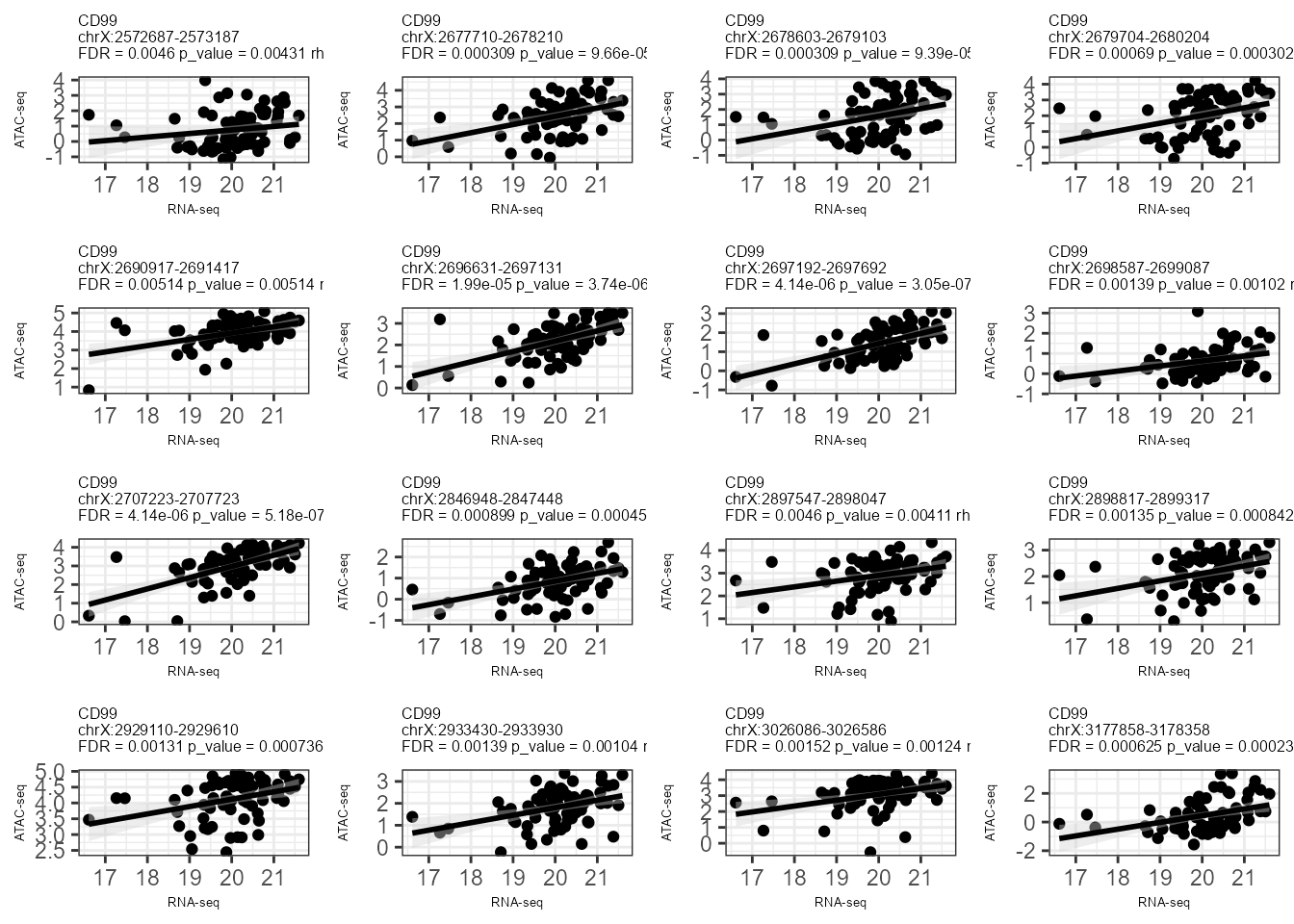

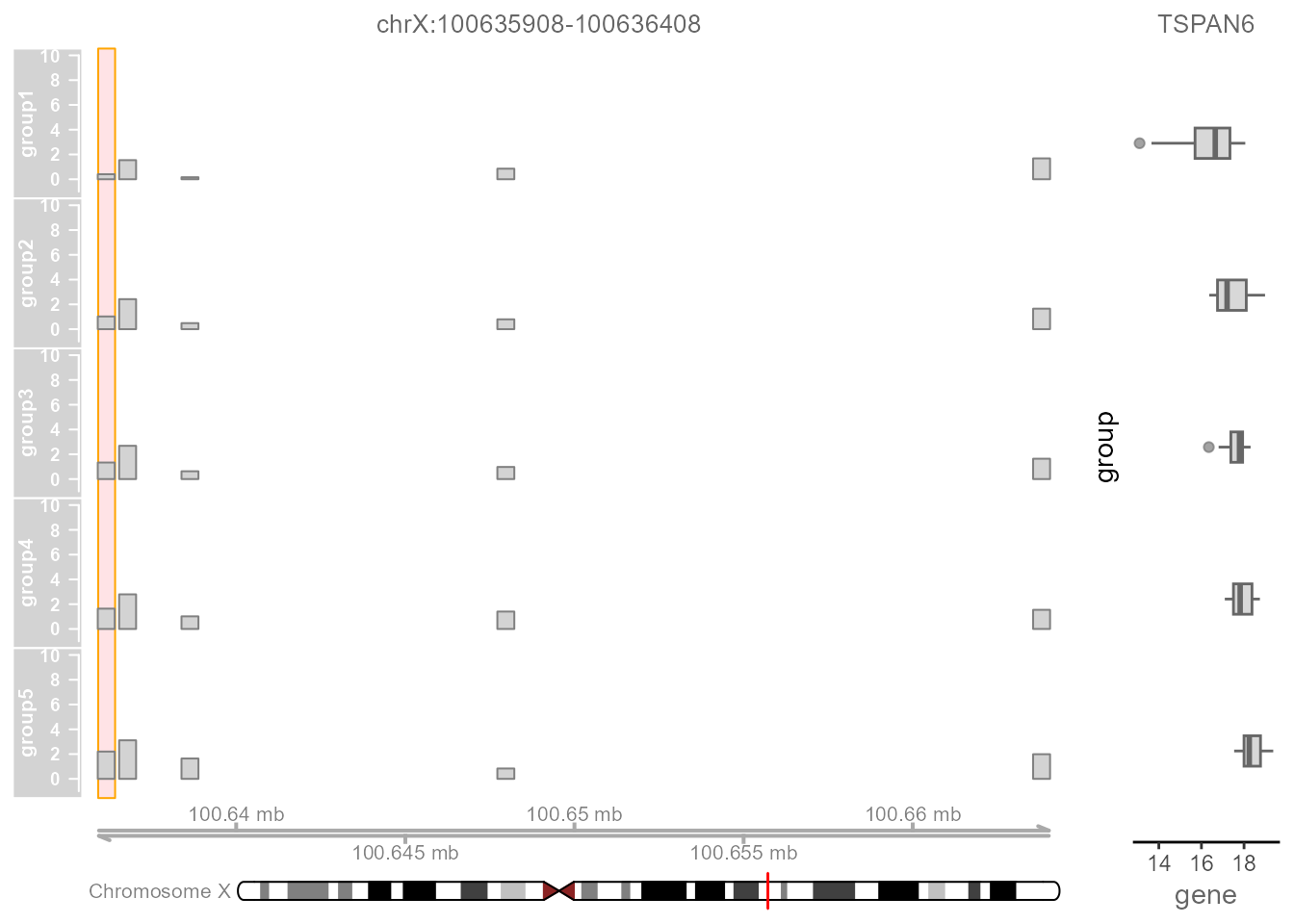
3.Regulatory Peaks Visualization

Now we can plot the Tn5 integration frequency and gene expression level across regions of the genome using the TrackPlot() function. For easier visualization, Linkage categorizes samples into five groups based on the quantitative chromatin accessibility of the specific regulatory peak from low to high. For each group, pseudo-bulk accessibility tracks and expression boxplot of the target gene can be viewed. Alongside these accessibility tracks we can visualize other important information including gene annotation and peak coordinates.

TrackPlot(
  LinkageObject,
  Geneid = "TSPAN6",
  peakid = "chrX:100635908-100636408",
  Species = "Homo"
)

4.Regulatory Peaks Annotation

Linkage can help you visualize the annotation of the predicational regulatory peaks. The PeakAnnotation() perform the annotation of all predicational regulatory peaks in terms of genomic location features, which includes whether the peak is in the TSS, Exon, 5' UTR, 3' UTR, Intronic or Intergenic and the position and strand information of the nearest gene of the peaks. You can produce the upsetplot for visualizing the overlaps and distribution in annotation for peaks by the AnnoUpsetPlot() function.

LinkageObject <- PeakAnnotation(LinkageObject, Species = "Homo")
AnnoUpsetPlot(LinkageObject = LinkageObject)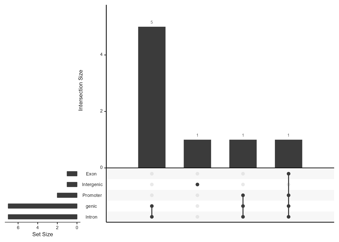

5.Motif Encichment Analysis

Next, you can visualize the enriched CREs within potential regulatory peaks by the MotifEnrichment() function. CREs and the TFs that binding on them play a central role in gene transcription regulation, which can be detected by ATAC-seq data. This function can help you view the location and binding score information of each enriched TFBS of the given DNA region.

library(DT)
df <- MotifEnrichment(LinkageObject@cor.peak$TSPAN6, "Homo")
brks1 <-
  quantile(df$score,
           probs = seq(.05, .95, .05),
           na.rm = TRUE)
DT::datatable(
  df,
  selection = "single",
  extensions = c("Scroller", "RowReorder"),
  option = list(
    rowReorder = TRUE,
    deferRender = TRUE,
    scrollY = 295,
    scroller = TRUE,
    scrollX = TRUE,
    searchHighlight = TRUE,
    orderClasses = TRUE,
    autoWidth = F
  )
) %>% formatStyle(
  names(df)[8],
  background = styleColorBar(range(brks1), 'lightblue'),
  backgroundSize = '90% 100%',
  backgroundRepeat = 'no-repeat',
  backgroundPosition = 'center'
)

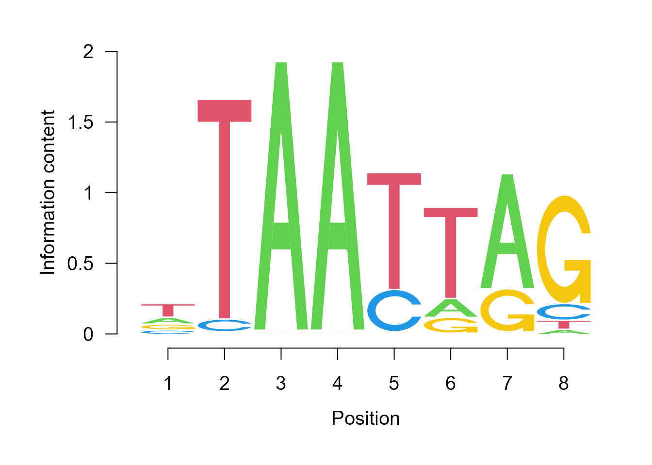
The SeqLogoPlot() function further help you to get the sequence logo of the given transcription factors.

SeqLogoPlot("MA0618.1")